Three-Dimensional CA

CellPyLib3d supports 3-dimensional cellular automata with periodic boundary conditions. The number of states, k, can be any whole number. The neighbourhood radius, r, can also be any whole number, and both Moore and von Neumann neighbourhood types are supported.

import cellpylib3d as cpl3d

# empty 3d grid
grid = cpl3d.init_simple3d(10, 10, 10, val=0) # init empty 3d grid

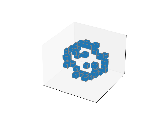
# oscilating shape from donut
grid[:, [3, 3, 3, 4, 4, 5, 5, 6, 6, 7, 7, 7], 4, [4, 5, 6, 3, 7, 3, 7, 3, 7, 4, 5, 6]] = 1

# evolve the CA for 20 time steps, using a 3d adaptation of Conway's Game of Life ruleset
grid = cpl3d.evolve3d(grid, timesteps=20, apply_rule=cpl3d.game_of_life_rule_3d)

cpl3d.plot3d(grid)

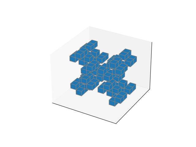
The image above represents the state at the final timestep. However, the state of the CA at any timestep can be visualized using the plot3d timestep argument. For example, in the code snippet below, the state at the 2nd timestep is plotted:

cpl3d.plot3d(grid, timestep=2)

Note that 2D CA can also be animated, so that the entire evolution of the CA can be visualized, using the plot3d_animate function:

cpl.plot3d_animate(grid)