Parallel CA

CellPyLib3d supports layering 2-dimensional automata to create 3-dimensional behaviour. The number of states, k, can be any whole number. The neighbourhood radius, r, applies to x and y components, but the z component extends the neighbourhood to cover all layers.

Note that parallel automata are constructed as 3D shapes, but require a list of rulesets, which are applied to respective layers of the automata.

import cellpylib3d as cpl3d

# empty 3d grid
grid = cpl3d.init_simple3d(10, 10, 10, val=0) # init empty 3d grid

# oscilating shape from donut
grid[:, [3, 3, 3, 4, 4, 5, 5, 6, 6, 7, 7, 7], 4, [4, 5, 6, 3, 7, 3, 7, 3, 7, 4, 5, 6]] = 1

# define rules for each layer
rules = [cpl3d.game_of_life_rule_parallel,] * 10

# evolve the CA for 20 time steps, using a 3d adaptation of Conway's Game of Life ruleset
grid = cpl3d.evolveParallel(grid, timesteps=20, apply_rules=rules)

cpl3d.plotParallel(grid)

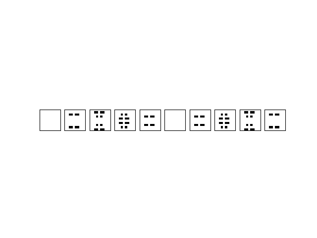
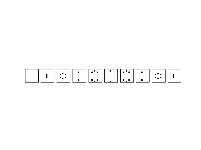
The image above represents the state at the final timestep. However, the state of the CA at any timestep can be visualized using the plotParallel timestep argument. For example, in the code snippet below, the state at the 2nd timestep is plotted:

cpl3d.plotParallel(grid, timestep=2)

Note that 3D CA can also be animated, so that the entire evolution of the CA can be visualized, using the plotParallel_animate function:

cpl.plotParallel_animate(grid)